


背景
ROC曲线是用于评估二分类模型性能的工具,它展示了模型在不同阈值下的真阳性率与假阳性率之间的关系,具体参考往期文章 实用机器学习技巧:使用ROC曲线进行多模型性能比较 ,但是标准的ROC并不能运用于多分类任务种,于是扩展出了宏平均ROC曲线
原理
宏平均ROC曲线是多分类问题中对ROC曲线的扩展,在多分类任务中,我们需要计算每一类别相对于其他所有类别的ROC曲线,然后对所有这些ROC曲线进行平均,从而得到宏平均ROC曲线,其主要步骤如下:
- 逐类计算ROC曲线:对于每个类别,将其视为正类,其他所有类别视为负类,计算出相应的ROC曲线,也就是可以看作对每个类别进行独热编码
- 计算AUC值:计算每个类别对应的AUC值
- 平均化:对所有类别的AUC值进行平均,从而得到宏平均AUC值,同时,将各类别的ROC曲线取平均,得到宏平均ROC曲线
宏平均ROC曲线的优点在于它平等地考虑了每个类别的性能,适用于类别数量不平衡的情况,不过,由于它对所有类别进行了简单平均,如果某些类别比其他类别更加重要,宏平均ROC可能无法完全反映分类器的实际性能
代码实现
数据读取
import pandas as pd

import numpy as np

import matplotlib.pyplot as plt

plt.rcParams['font.sans-serif'] = 'SimHei' # 设置中文显示

plt.rcParams['axes.unicode_minus'] = False

df = pd.read_excel('宏平均ROC曲线.xlsx')

df
该多分类数据存在5个类别
数据预处理
from sklearn.preprocessing import MinMaxScaler, label_binarize

from sklearn.model_selection import train_test_split

# 划分特征和目标变量

X = df.drop(['Type_encoded'], axis=1)

y = df['Type_encoded']

# 划分训练集和测试集

xtrain, xtest, ytrain, ytest = train_test_split(X, y, test_size=0.3,

                                                random_state=8,stratify=df['Type_encoded'])

# 标准化数据

scaler = MinMaxScaler()

xtrain_s = scaler.fit_transform(xtrain)

xtest_s = scaler.transform(xtest)
对数据集进行特征和目标变量的划分,并通过分层抽样划分为训练集和测试集,然后对特征数据进行了MinMax标准化处理
模型建立
from sklearn.ensemble import RandomForestClassifier


# 使用随机森林建模

model_rf = RandomForestClassifier(n_estimators=100, criterion='gini', bootstrap=True, max_depth=3, random_state=8)

model_rf.fit(xtrain_s, ytrain)
使用随机森林分类器(RandomForestClassifier)对标准化后的训练数据进行建模,并使用训练集进行拟合,以便后续对新数据进行预测,模型的参数指定了100棵树(n_estimators=100)、使用Gini系数作为划分标准(criterion='gini'),使用自助法(bootstrap=True),最大树深为3(max_depth=3),并设置了随机种子以保证结果的可重复性(random_state=8)
模型评价
详细指标
from sklearn.metrics import classification_report


# 预测测试集

y_pred = model_rf.predict(xtest_s)


# 输出模型报告, 查看评价指标

print(classification_report(ytest, y_pred))
混淆矩阵热力图
from sklearn.metrics import confusion_matrix

import seaborn as sns

# 输出混淆矩阵

conf_matrix = confusion_matrix(ytest, y_pred)


# 绘制热力图

plt.figure(figsize=(10, 7), dpi=1200)

sns.heatmap(conf_matrix, annot=True, annot_kws={'size':15},

            fmt='d', cmap='YlGnBu', cbar_kws={'shrink': 0.75})

plt.xlabel('Predicted Label', fontsize=12)

plt.ylabel('True Label', fontsize=12)

plt.title('Confusion matrix heat map', fontsize=15)

plt.show()
宏平均ROC绘制
宏平均ROC计算
from sklearn import metrics

# 预测并计算概率

ytest_proba_rf = model_rf.predict_proba(xtest_s)


# 将y标签转换成one-hot形式

ytest_one_rf = label_binarize(ytest, classes=[0, 1, 2,3,4])


# 宏平均法计算AUC

rf_AUC = {}

rf_FPR = {}

rf_TPR = {}


for i in range(ytest_one_rf.shape[1]):

    rf_FPR[i], rf_TPR[i], thresholds = metrics.roc_curve(ytest_one_rf[:, i], ytest_proba_rf[:, i])

    rf_AUC[i] = metrics.auc(rf_FPR[i], rf_TPR[i])

print(rf_AUC)


# 合并所有的FPR并排序去重

rf_FPR_final = np.unique(np.concatenate([rf_FPR[i] for i in range(ytest_one_rf.shape[1])]))


# 计算宏平均TPR

rf_TPR_all = np.zeros_like(rf_FPR_final)

for i in range(ytest_one_rf.shape[1]):

    rf_TPR_all += np.interp(rf_FPR_final, rf_FPR[i], rf_TPR[i])

rf_TPR_final = rf_TPR_all / ytest_one_rf.shape[1]


# 计算最终的宏平均AUC

rf_AUC_final = metrics.auc(rf_FPR_final, rf_TPR_final)

AUC_final_rf = rf_AUC_final  # 最终AUC


print(f"Macro Average AUC with Random Forest: {AUC_final_rf}")
利用随机森林模型对测试集进行预测,并计算每个类别的预测概率。然后,将实际标签 ytest 转换为 one-hot 编码形式,以便进行多分类的 ROC 曲线分析,接着,通过逐类别计算 ROC 曲线和 AUC 值,并保存到字典中,最后,通过合并所有类别的 FPR 值并计算宏平均 TPR,从而得到最终的宏平均 AUC 值,用于评估随机森林模型在多分类任务中的整体性能
可视化输出
plt.figure(figsize=(10, 5), dpi=300)

# 使用不同的颜色和线型

plt.plot(rf_FPR[0], rf_TPR[0], color='#1f77b4', linestyle='-', label='Class 1 ROC  AUC={:.4f}'.format(rf_AUC[0]), lw=2)

plt.plot(rf_FPR[1], rf_TPR[1], color='#ff7f0e', linestyle='-', label='Class 2 ROC  AUC={:.4f}'.format(rf_AUC[1]), lw=2)

plt.plot(rf_FPR[2], rf_TPR[2], color='#2ca02c', linestyle='-', label='Class 3 ROC  AUC={:.4f}'.format(rf_AUC[2]), lw=2)

plt.plot(rf_FPR[3], rf_TPR[3], color='#d62728', linestyle='-', label='Class 4 ROC  AUC={:.4f}'.format(rf_AUC[3]), lw=2)

plt.plot(rf_FPR[4], rf_TPR[4], color='#9467bd', linestyle='-', label='Class 5 ROC  AUC={:.4f}'.format(rf_AUC[4]), lw=2)

# 宏平均ROC曲线

plt.plot(rf_FPR_final, rf_TPR_final, color='#000000', linestyle='-', label='Macro Average ROC  AUC={:.4f}'.format(rf_AUC_final), lw=3)

# 45度参考线

plt.plot([0, 1], [0, 1], color='gray', linestyle='--', lw=2, label='45 Degree Reference Line')

plt.xlabel('False Positive Rate (FPR)', fontsize=15)

plt.ylabel('True Positive Rate (TPR)', fontsize=15)

plt.title('Random Forest Classification ROC Curves and AUC', fontsize=18)

plt.grid(linestyle='--', alpha=0.7)

plt.legend(loc='lower right', framealpha=0.9, fontsize=12)

plt.savefig('RF_optimized.pdf', format='pdf', bbox_inches='tight')

plt.show()
绘制随机森林分类器在多分类任务中的 ROC 曲线,并计算并展示了每个类别的 AUC 值以及宏平均 ROC 曲线的 AUC
往期推荐
利用XGBoost模型进行多分类任务下的SHAP解释附代码讲解及GUI展示
快速选择最佳模型:轻松上手LightGBM、XGBoost、CatBoost和NGBoost!
小白轻松上手:一键生成SHAP解释图的GUI应用,支持多种梯度提升模型选择
综合多种梯度提升模型:LightGBM、XGBoost、CatBoost与NGBoost的集成预测
微信号|deep_ML
欢迎添加作者微信进入Python、ChatGPT群
进群请备注Python或AI进入相关群
无需科学上网、同步官网所有功能、使用无限制
如果你对类似于这样的文章感兴趣。
欢迎关注、点赞、转发~
个人观点,仅供参考